Power BI Data Analyst PL-300
Data Modeling and Dimensional Schema Design
The data model is the architectural backbone of every Power BI solution. Every visual, every DAX measure, and every report filter resolves through the relationships and cardinalities defined in the model layer. This chapter examines the dimensional modeling patterns that dominate the PL-300 exam: star and snowflake schemas, relationship cardinality rules, filter propagation behavior, role-playing dimensions, and the requirements for a properly marked date table.
1. Foundations of Dimensional Modeling
Why Dimensional Modeling Matters for PL-300
Dimensional modeling organizes data into two entity types: fact tables (quantitative, transactional data such as sales amounts and order quantities) and dimension tables (descriptive attributes such as product names, customer geographies, and calendar dates). The model structure directly determines DAX performance, filter propagation correctness, and long-term maintainability.
A poorly structured model — flat tables with repeated attributes or incorrectly configured cardinalities — forces increasingly complex DAX to compensate. A clean dimensional model lets even simple measures return correct, high-performing results across all filter contexts. Microsoft explicitly recommends the star schema as the default approach for analytical models in Power BI.
Anatomy of a Star Schema
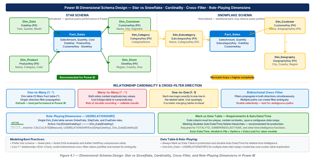
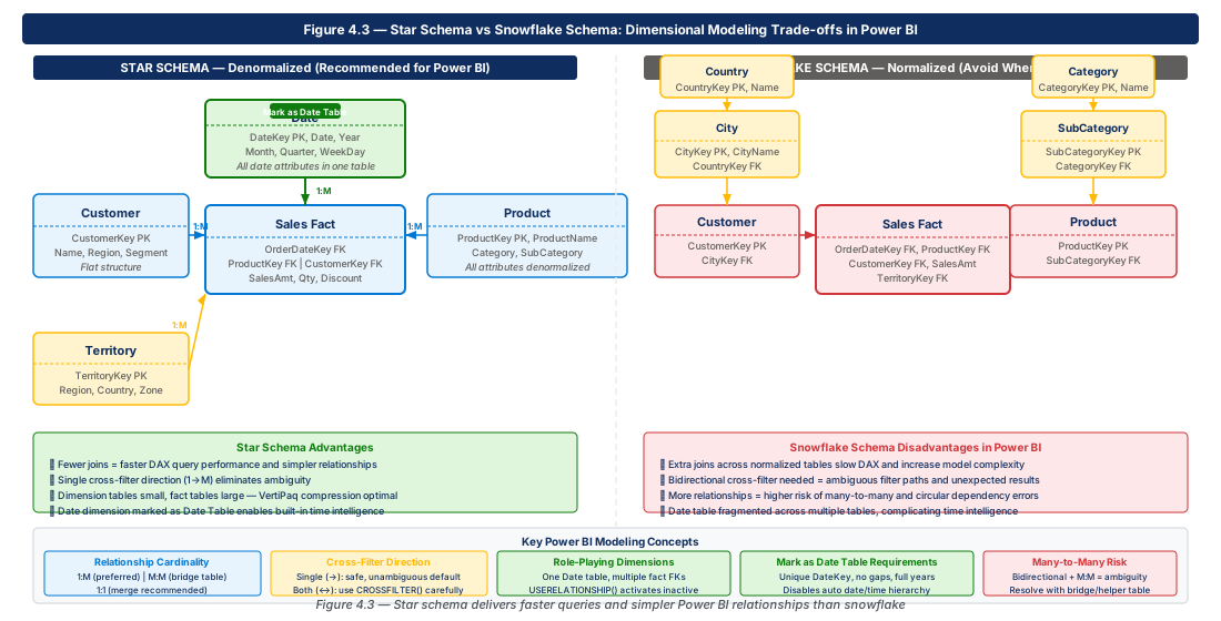
A star schema places a single fact table at the center, surrounded by dimension tables connected through one-to-many relationships. The fact table (FactSales) holds foreign key columns (DateKey, CustomerKey, ProductKey) plus numeric measures (SalesAmount, OrderQuantity). When a user slices by DimProduct[Category], Power BI filters DimProduct and propagates that filter into FactSales — no additional DAX required.
The star schema minimizes relationship traversal count (faster queries), presents semantically clear field lists for report authors, and makes CALCULATE filter arguments predictable because all dimension attributes maintain a one-to-many relationship to the fact.
Note
The star schema is the default recommended modeling pattern per Microsoft's documentation. When an exam question presents a modeling scenario with no additional constraints, a star schema answer is nearly always preferred.
Snowflake Schema: When and Why
A snowflake schema normalizes dimensions into sub-dimensions — for example, separating DimProduct into DimProduct and DimProductCategory. In classic row-store warehouses this reduced storage redundancy, but Power BI's VertiPaq engine compresses repeated string values via dictionary encoding, making denormalization essentially free from a storage perspective.
Each additional table hop adds query overhead. A filter on DimProductCategory must traverse two relationships before reaching FactSales. Microsoft recommends using Power Query's Merge Queries to flatten snowflake sub-dimensions into their parent dimension tables before loading to the model.
Tip
When you receive a snowflake-structured source in Power Query, use Merge Queries to join sub-dimensions into the parent dimension. The result is a star schema that performs better and is easier to maintain.
2. Schema Design Comparison and Decision Framework
Star vs. Snowflake Trade-off Analysis
| Dimension | Star Schema | Snowflake Schema |
|---|---|---|
| Table count | Lower — one table per dimension | Higher — sub-dimensions add tables |
| VertiPaq storage | Minimal increase due to compression | Marginal benefit in practice |
| Query performance | Faster — fewer relationship hops | Slower — each sub-dimension adds traversal |
| DAX complexity | Low — predictable filter context | Higher — cross-table filters require more care |
| Recommended for Power BI | Yes — Microsoft default | Only when source cannot be denormalized |
| Maintenance burden | Lower — fewer tables | Higher — changes span multiple tables |
Flat Table Anti-Pattern
A flat table model combines fact and dimension attributes into a single wide table — for example, a Sales table containing CustomerName, ProductName, CategoryName, SalesAmount, and millions of rows. VertiPaq cannot compress long repeating string columns efficiently without the integer key separation a star schema provides, causing severe memory and performance problems.
Beyond storage, the flat table breaks DAX relationship semantics: there are no relationships to traverse, so every filter must be expressed as explicit FILTER or CALCULATETABLE expressions — making measures brittle and hard to maintain.
Warning
Identify flat table models in exam questions by looking for dimension attributes (names, descriptions, categories) mixed with numeric measure columns in a single millions-row table. Refactoring to a star schema is the correct answer.
3. Relationship Cardinality and Filter Direction
One-to-Many Relationships: The Foundation
A one-to-many relationship connects the primary key of a dimension (the "one" side) to the foreign key of a fact table (the "many" side). Filter propagation flows by default from dimension to fact — a product category slicer filters DimProduct and that filter propagates into FactSales automatically.
Common exam failure modes: a dimension table with duplicate key values (Power BI reclassifies the relationship as many-to-many), and fact rows with unmatched dimension keys (grouped under a blank member in the dimension, potentially inflating totals).
Important
Power BI does not reject fact rows with unmatched dimension keys — it groups them under a blank member. Always validate referential integrity between fact and dimension key columns during model build.
Many-to-Many Relationships: Patterns and Pitfalls
Many-to-many relationships arise in two scenarios. The first is a genuine business many-to-many (e.g., customers and loyalty product memberships) — resolve with a bridge table that decomposes the relationship into two one-to-many joins. The second is a shared dimension across multiple fact tables at different grains — resolve with a conformed dimension using one-to-many relationships from the dimension to each fact.
Note
Power BI displays a double asterisk (**) on both ends of a many-to-many relationship line, "1" on the dimension side and "*" on the fact side for one-to-many. These visual indicators are tested on the PL-300 exam.
One-to-One Relationships: Use Cases and Risks
One-to-one relationships exist when both join columns contain only unique values. They are uncommon in analytical models and typically indicate a horizontally partitioned dimension or an RLS user-mapping table. In most cases the correct exam answer is to merge the two tables in Power Query, eliminating the relationship and its traversal overhead.

4. Bidirectional Cross-Filter and Ambiguity Resolution
How Bidirectional Filtering Works
By default, filters propagate from the "one" side to the "many" side. Enabling bidirectional cross-filtering on a relationship (indicated by a double-headed arrow in Model view) allows propagation in both directions. A common use case is a many-to-many scenario resolved through a bridge table where you want a product filter to also filter the customer slicer.
Ambiguity and the Danger of Circular Paths
When bidirectional filters are enabled on multiple relationships, Power BI may find multiple valid propagation paths to reach a target table — creating ambiguity. The engine will disable one of the conflicting relationships and display a warning in Model view, or silently return incorrect results.
Warning
Enabling bidirectional cross-filtering on multiple relationships is one of the most common causes of incorrect DAX results. Always evaluate whether a DAX-based solution using CROSSFILTER can achieve the same goal with greater control.
DAX-Based Filter Direction with CROSSFILTER
CROSSFILTER(LeftColumn, RightColumn, CrossFilterType) changes filter direction only within the evaluation context of a specific measure, giving precise measure-level control. CrossFilterType accepts Both, OneWay, OneWayRightFiltersLeft, or None.
-- Count distinct products for customers filtered in the current context
DistinctProductsByCustomer =
CALCULATE(
    DISTINCTCOUNT(FactSales[ProductKey]),
    CROSSFILTER(DimCustomer[CustomerKey], FactSales[CustomerKey], Both)
)
5. Role-Playing Dimensions and USERELATIONSHIP
The Role-Playing Dimension Pattern
A role-playing dimension is a single dimension table used multiple times in a fact table for different business roles. The canonical example is DimDate relating to FactSales[OrderDateKey], FactSales[ShipDateKey], and FactSales[DueDateKey]. Power BI allows only one active relationship between any two tables — configure the most common role (typically order date) as active; the remaining roles become inactive relationships shown as dashed lines in Model view.
Note
Inactive relationships display as dashed lines in Model view; active relationships display as solid lines. A table pair can have multiple inactive relationships but only one active relationship — a frequently tested PL-300 visual distinction.
Implementing USERELATIONSHIP in DAX
USERELATIONSHIP is used exclusively inside CALCULATE or CALCULATETABLE. It activates an inactive relationship for the duration of the enclosing evaluation context, automatically deactivating the currently active relationship between the same table pair.
-- Sales amount via the ShipDate role instead of the default OrderDate role
ShipDateSalesAmount =
CALCULATE(
    SUM(FactSales[SalesAmount]),
    USERELATIONSHIP(DimDate[DateKey], FactSales[ShipDateKey])
)
Fact rows with null values in the inactive role's key column (e.g., unshipped orders with a null ShipDateKey) are excluded from the filter result when that relationship is active — correct behavior but a subtle filter characteristic that exam questions test explicitly.
Duplicating the Dimension as an Alternative
An alternative is to import DimDate multiple times in Power Query, naming each copy for its role (DimOrderDate, DimShipDate), each with a single active relationship. This eliminates USERELATIONSHIP from every measure and makes role intent visually clear. For small dimensions like date tables (typically 3,650 rows per decade), the memory penalty of duplication is trivial.
Tip
For date dimensions with 2–4 roles, duplicating into named role-playing copies is often cleaner than requiring every measure to use USERELATIONSHIP. For large dimensions with many roles, inactive relationships conserve memory.
6. Mark as Date Table Requirements and Auto Date/Time
The Auto Date/Time Feature
Power BI Desktop automatically creates a hidden date table for every date or date/time column detected in the model, enabling the built-in Year/Quarter/Month/Day hierarchy. For simple models this is convenient, but in production models with many fact tables and date columns, the hidden Auto Date/Time tables can consume as much memory as all user-visible tables combined.
Warning
Always disable Auto Date/Time (File > Options > Data Load > Time Intelligence > Auto Date/Time) when you have implemented a properly marked date table to eliminate hidden memory overhead.
Mark as Date Table Requirements
To designate a table as the authoritative date dimension for time intelligence DAX functions, right-click it in Model view and select Mark as date table. The specified date column must satisfy four requirements tested on the PL-300 exam:
- Data type must be Date or DateTime (not text, not integer).
- Column must contain no blank or null values.
- Column must contain no duplicate date values.
- Column must be contiguous — no gaps between the minimum and maximum dates.
Important
The contiguous date requirement is the most frequently violated in practice. A date table built from distinct fact dates will skip weekends and holidays, causing time intelligence functions like DATESINPERIOD to return incorrect results.
Building a Compliant Date Table
Use Power Query's List.Dates function to generate every calendar date in the required range without gaps, then add calendar attribute columns for year, quarter, month name, weekday, and fiscal periods.
// Generate a complete, contiguous date table from 2020-01-01 to today
let
    StartDate = #date(2020, 1, 1),
    EndDate   = Date.From(DateTime.LocalNow()),
    DateList  = List.Dates(StartDate, Duration.Days(EndDate - StartDate) + 1, #duration(1,0,0,0)),
    DateTable = Table.FromList(DateList, Splitter.SplitByNothing(), {"Date"}),
    TypedTable = Table.TransformColumnTypes(DateTable, {{"Date", type date}}),
    AddYear   = Table.AddColumn(TypedTable, "Year", each Date.Year([Date]), Int64.Type),
    AddMonth  = Table.AddColumn(AddYear, "MonthName", each Date.ToText([Date], "MMMM"), type text)
in
    AddMonth
7. Lab
CE-07: Provision Synapse Analytics for Star Schema Modeling
Create the Azure infrastructure — resource groups, ADLS Gen2 storage, Synapse workspace, and dedicated SQL pool — that will serve as the dimensional model source for Power BI.
RG="rg-data-modeling-dimensional-schema-prod-001"
WS="data-modeling-prod-eastus2-001"
SA="stardataprod001"
az group create --name "$RG" --location eastus2
az storage account create --name "$SA" --resource-group "$RG" --hierarchical-namespace true
az synapse workspace create --name "$WS" --resource-group "$RG" \
  --storage-account "$SA" --file-system synapse-data \
  --sql-admin-login-user synapseadmin --sql-admin-login-password "$SQL_PWD"
az synapse sql pool create --name sqldwprod001 --performance-level DW100c \
--workspace-name "$WS" --resource-group "$RG"CE-08: Deploy Star Schema DDL and Validate DimDate Integrity
Execute the star schema DDL script in the Synapse dedicated SQL pool, populate DimDate with contiguous dates, and validate that the date table meets all Mark as Date Table requirements before deploying the Power BI dataset.
# Deploy DDL and validate DimDate integrity
az synapse sql-script run --workspace-name "$WS" --name create-star-schema-ddl \
  --resource-group "$RG"
az synapse pipeline run --workspace-name "$WS" \
  --name populate-dimdate-pipeline --resource-group "$RG"
# Validate: TotalRows == DistinctDates == ExpectedContiguousDays, NullCount == 0
az synapse sql-script run --workspace-name "$WS" \
  --name validate-dimdate-integrity --resource-group "$RG"
8. Chapter Summary
| Concept | Key Exam Point |
|---|---|
| Star schema | Recommended pattern: one fact, one-to-many dimension tables, fewest hops, simplest DAX filter context |
| Snowflake schema | Avoid in Power BI; denormalize sub-dimensions via Power Query Merge to reduce relationship traversal |
| One-to-many cardinality | Foundational relationship type; filters flow from dimension (1) to fact (*) by default |
| Many-to-many cardinality | Resolve with bridge table (business M:M) or conformed dimension (shared dimension across facts) |
| Bidirectional cross-filter | Risks ambiguous paths; prefer scoped CROSSFILTER in DAX over permanent model-level setting |
| USERELATIONSHIP | Activates an inactive relationship within CALCULATE; used for non-default date roles |
| Mark as Date Table | Date type, no nulls, no duplicates, contiguous range; disable Auto Date/Time after marking |
Chapter: 4 of 12 | Status: v0.1 Draft |